How It Works
The pipeline transforms raw geospatial data into actionable site recommendations in six stages.
Five geospatial data modalities are acquired and harmonised into EPSG:27700 (British National Grid): population (LandScan), demographics (Census 2021), crime (police.uk 2021), transport (OSM stations + Overpass bus stops), and POIs (OSMnx).
Three Data Modalities
| Modality | Representation | Example | Precision |
|---|---|---|---|
| Vector | Discrete geometric primitives with exact coordinate pairs | OSM cafe locations (Points), building footprints (Polygons) | Sub-metre |
| Raster | Regular grid of cells, each storing a numeric value | LandScan population grid — each pixel holds a count | ~1 km per pixel |
| Tabular | Attribute records keyed by a spatial identifier | ONS Census CSVs — percentages per Output Area | OA centroid |
POI Categorisation
Each Point of Interest is classified into a business role relative to the target business type:
| Role | OSM Tags (examples) | Effect on Score |
|---|---|---|
| Competitor | Same type as target (e.g. cafes for cafe model) | Excluded from features (encodes the target) |
| Synergy | gym, university, office, library, co-working | Increases score (complementary foot traffic) |
| Anchor | station (public transport) | Increases score (transit node) |
| Other | bakery, supermarket, restaurant | Contextual enrichment |
Competition Density (k=2 Ring)
For each business type, a competition density feature counts same-type businesses in a k=2 H3 ring (~18 neighboring hexagons, ~350m radius).
Census Merge
Three ONS Census 2021 CSVs (Economic Activity, Age Structure, Qualifications) are merged
on geog_code (Output Area identifier), producing 846 OAs with 7 demographic columns.
Missing values are imputed with the column median.
Exploratory Data Analysis
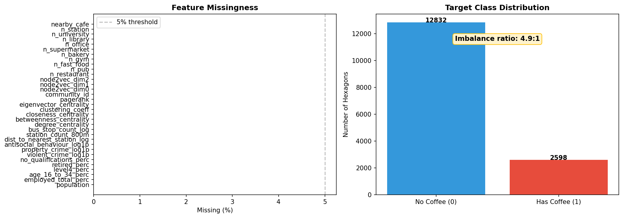
Fig. 1 — Feature missingness audit (left) and target class distribution (right).
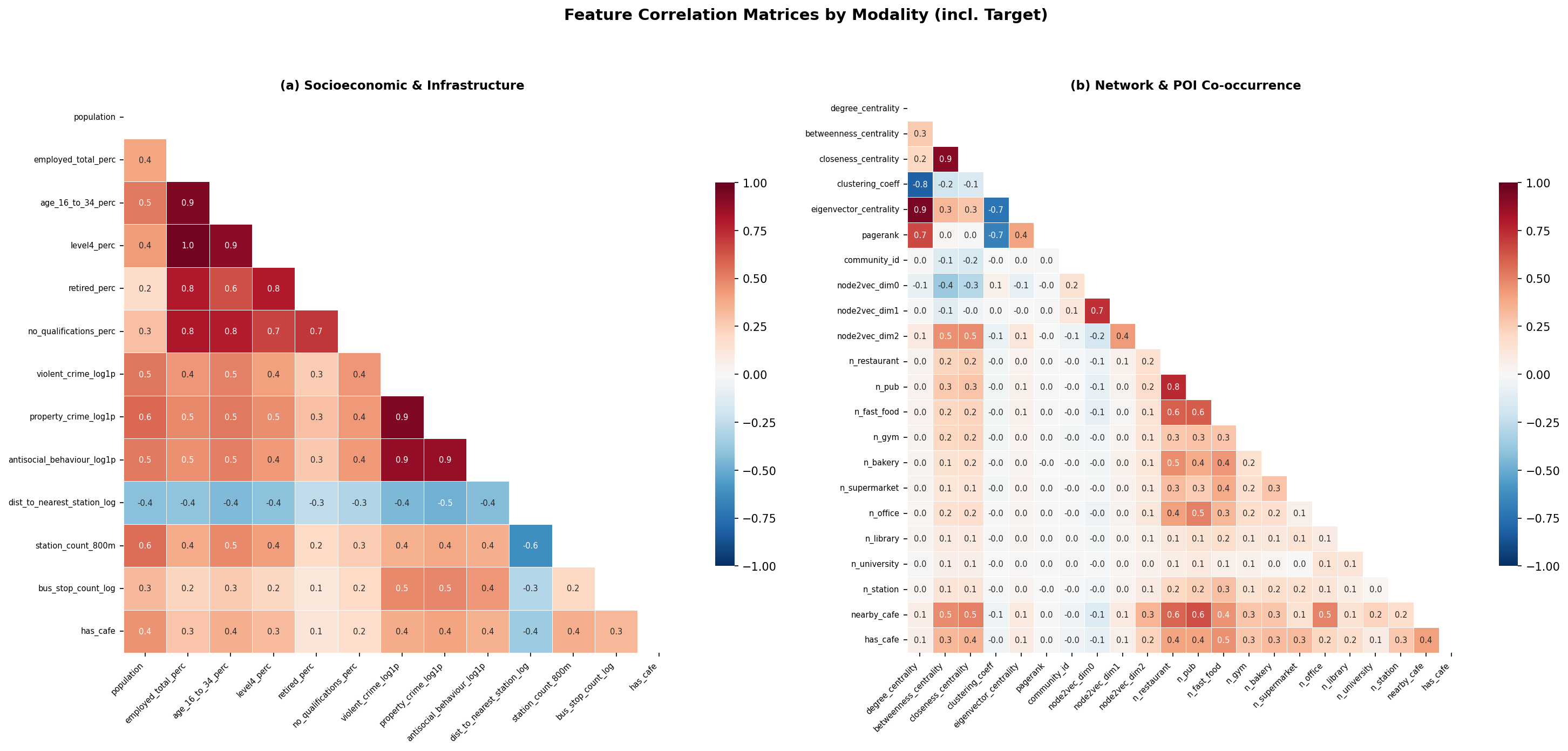
Fig. 2 — Feature correlation matrix.
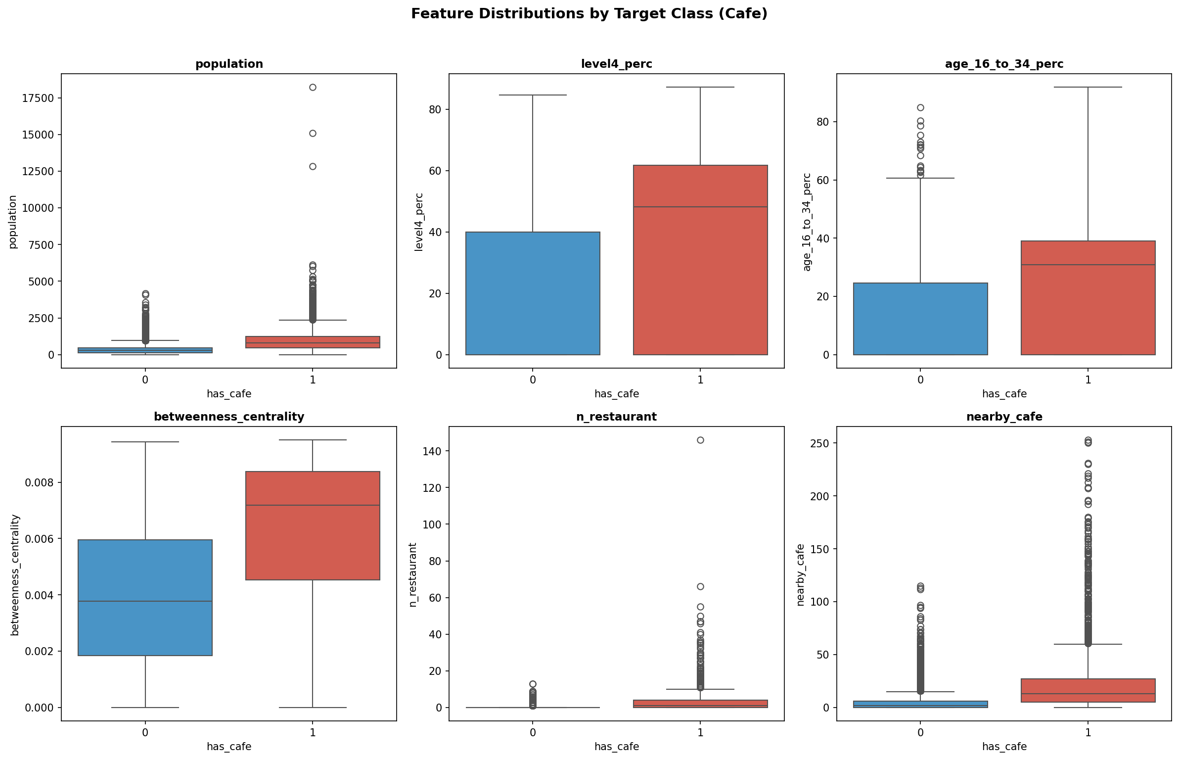
Fig. 3 — Feature distributions split by target class (cafe).
Uber's H3 library partitions Greater London into hierarchical hexagonal cells. Unlike square grids, hexagons have 6 equidistant neighbours — ideal for walking-distance analysis.
Why Resolution 9?
| Resolution | Edge Length | Hex Area | Use Case |
|---|---|---|---|
| 7 | ~1.2 km | ~5.16 km² | District-level |
| 8 | ~460 m | ~0.74 km² | Neighbourhood |
| 9 | ~174 m | ~0.105 km² | Walking-scale (our choice) |
| 10 | ~66 m | ~0.015 km² | Street-level |
At Resolution 9, each hexagon covers roughly the area a person walks in 2 minutes — the micro-unit of the 15-minute city (Moreno et al., 2021).
Enrichment Pipeline
Census demographics are joined via sjoin_nearest with population-weighted mean
aggregation. Hexes with no OA match receive the borough median (conservative imputation).
Street-level crime data from police.uk (Metropolitan Police + City of London Police, ~1.08M raw records across 2021) is cleaned, deduplicated, and aggregated to H3 hexagons.
Data Cleaning
The raw data contains significant quality issues that are resolved before feature engineering:
| Issue | Scale | Action |
|---|---|---|
| Exact duplicate rows | ~166,000 (15.7%) | Removed via deduplication |
| Crime ID duplicates | ~40,600 | Jurisdictional overlap at force boundaries; deduplicated by Crime ID |
| Non-London records | ~19,800 | Met Police covers some edge areas (Epping, Elmbridge); filtered by LSOA to 33 boroughs |
| ASB without Crime ID | ~302,000 | By design in police.uk data; retained after exact dedup |
Post-cleaning: ~852,000 verified crime records across all 33 London boroughs.
Crime Type Grouping
14 raw crime types grouped into 3 retail-relevant categories:
| Group | Types Included | Retail Signal |
|---|---|---|
| Violent crime | Violence, Robbery, Weapons, Public order, Drugs | Safety perception — deters footfall |
| Property crime | Burglary, Vehicle crime, Theft, Shoplifting, Criminal damage | Operational cost — shrinkage, insurance |
| Anti-social behaviour | ASB | Neighbourhood quality — high street decline |
Features (3 per Hexagon)
Each crime group is aggregated per hex, then log-transformed (log1p) to compress
the right-skewed tail — hotspot hexes like Oxford Street and Stratford Westfield have thousands of incidents
while most residential hexes have single digits. Hexes with no crime receive 0
(an observed zero, not imputed with borough median).
| Feature | Description |
|---|---|
violent_crime_log1p | log(1 + violent crime count) — safety signal |
property_crime_log1p | log(1 + property crime count) — retail cost signal |
antisocial_behaviour_log1p | log(1 + ASB count) — neighbourhood quality signal |
Transport connectivity features capture the accessibility gradient that drives retail footfall.
Station data comes from the existing POI fetch (public_transport=station);
bus stops are fetched separately via Overpass API (highway=bus_stop, ~19,000 across London).
Spatial Computation
All distance calculations use EPSG:27700 (British National Grid) for metric accuracy.
A scipy.spatial.cKDTree indexes station locations for O(log n) nearest-neighbour and
radius queries against ~16,000 hex centroids.
Features (3 per Hexagon)
| Feature | Description |
|---|---|
dist_to_nearest_station_log | log(1 + BNG meters to nearest rail/tube/DLR station) — accessibility gradient |
station_count_800m | Count of stations within 800m walkable catchment — interchange density |
bus_stop_count_log | log(1 + bus stops per hex) — local transit frequency proxy |
Missing Values
Bus stops: 0 for hexes with no stops (observed zero). Station distance: always computed (no missing values). Station count: 0 when no stations within 800m.
The enriched H3 grid becomes a spatial graph where hexagons are nodes and edges connect adjacent hexes. From this graph we extract three layers of structural information.
Six Centrality Metrics
| Metric | What It Measures | Business Meaning |
|---|---|---|
| Degree | Number of neighbours | Interior (6) vs boundary (<6) connectivity |
| Betweenness | Frequency on shortest paths | Transit corridor importance |
| Closeness | Average distance to all nodes | Central vs peripheral location |
| Clustering | Neighbour interconnection | Neighbourhood cohesion |
| Eigenvector | Influence via well-connected neighbours | Hub proximity (near other hubs) |
| PageRank | Damped random walk steady state | Foot-traffic accumulation potential |
Louvain Community Detection
The Louvain algorithm partitions the H3 adjacency graph
into communities, maximising modularity. Each hexagon receives a community_id
capturing which spatial neighbourhood cluster it belongs to.
Node2Vec Graph Embeddings
Node2Vec learns a 3-dimensional vector representation for each hexagon by simulating biased random walks on the graph. Hexagons with similar graph neighbourhoods receive similar embeddings, even if geographically distant.
Heuristic Site Score
Where DH = Level 4 qualification % / 100 (demand proxy), S = synergy count, A = anchor count, C = competitor count.
Problem Formulation
Binary classification: for each of 6 business types, predict whether a hexagon should contain that business. The commercially valuable output is the False Positives — locations predicted as suitable that have no current supply.
Feature Matrix (33 Features per Business Type)
| Modality | Count | Features |
|---|---|---|
| Footfall | 1 | population (LandScan zonal sum) |
| Demographics | 5 | employed_total_perc, age_16_to_34_perc, level4_perc, retired_perc, no_qualifications_perc |
| Crime Rates | 3 | violent_crime_log1p, property_crime_log1p, antisocial_behaviour_log1p |
| Transport Access | 3 | dist_to_nearest_station_log, station_count_800m, bus_stop_count_log |
| Graph Centrality | 6 | degree_centrality, betweenness_centrality, closeness_centrality, clustering_coeff, eigenvector_centrality, pagerank |
| Community Structure | 1 | community_id (Louvain) |
| Graph Embeddings | 3 | node2vec_dim0/1/2 |
| POI Co-occurrence | 10 | Counts of all 11 POI types except the target type |
| Competition Density | 1 | nearby_{type} — same-type businesses in k=2 ring |
Spatial Cross-Validation
Standard k-fold CV violates spatial independence. We group Resolution-9 hexes by their Resolution-7 parent cell (~0.74 km² blocks). All hexes sharing a parent are assigned to the same fold, preserving spatial integrity across 5 folds.
Model Comparison
| Model | Type | Imbalance Handling | Rationale |
|---|---|---|---|
| Logistic Regression | Linear | class_weight='balanced' | Interpretable baseline |
| Random Forest | Bagged ensemble | class_weight='balanced' | Non-linear, robust |
| XGBoost | Boosted ensemble | scale_pos_weight | State-of-the-art tabular |
Evaluation Figures
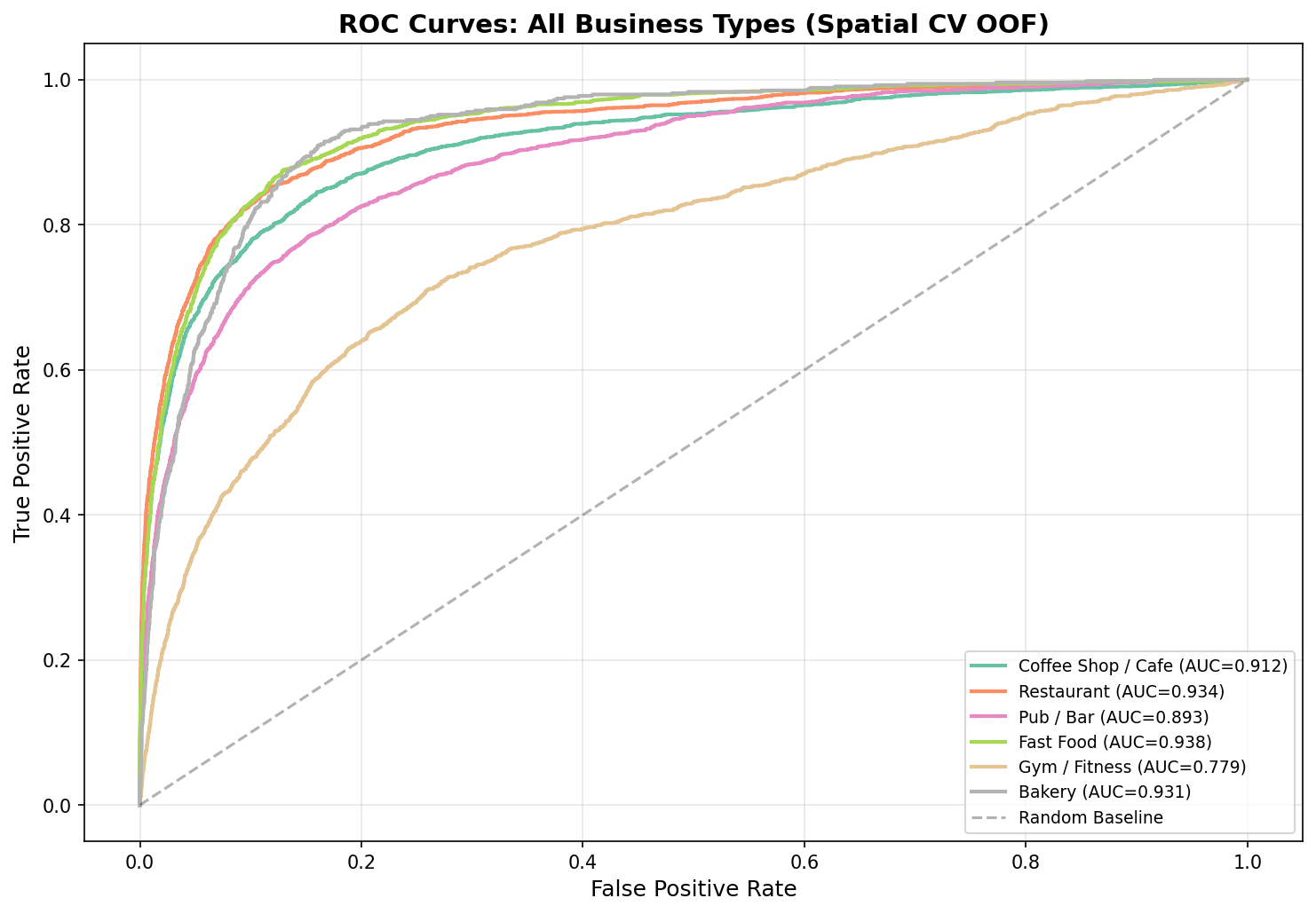
Fig. 4 — ROC curves (out-of-fold, spatial CV)
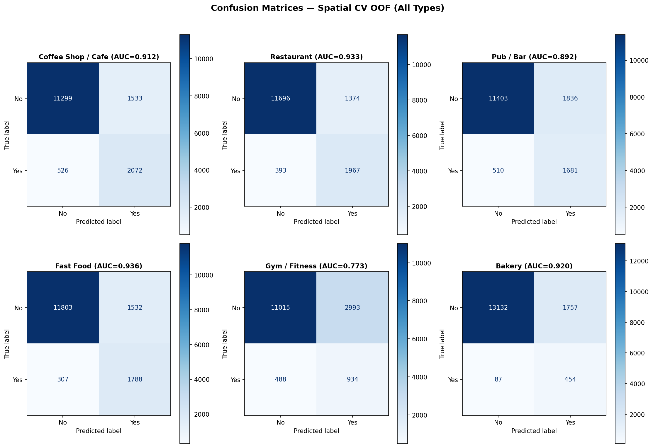
Fig. 5 — Confusion matrices (out-of-fold, all 6 types)
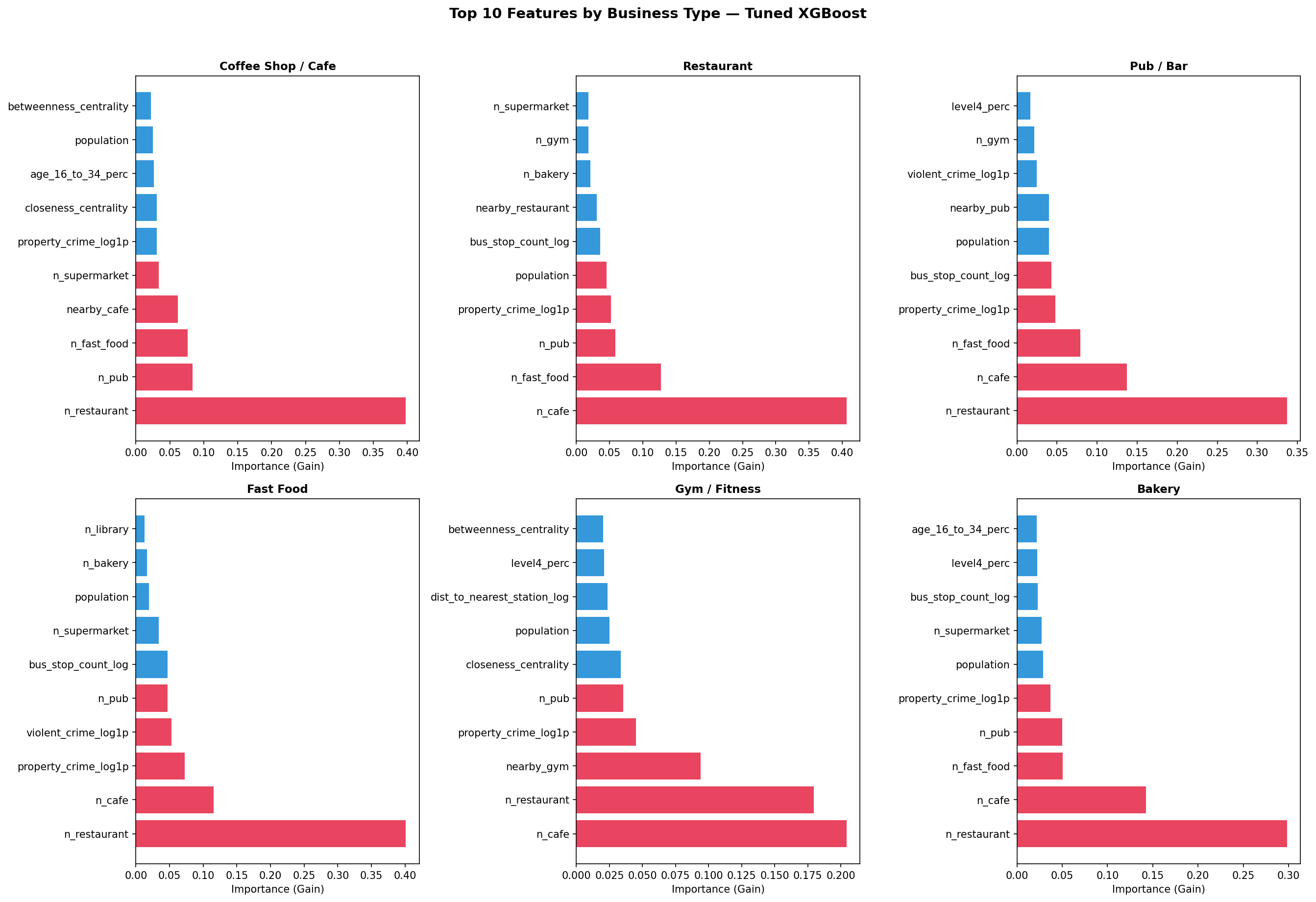
Fig. 6 — Top 10 features by business type (XGBoost gain)
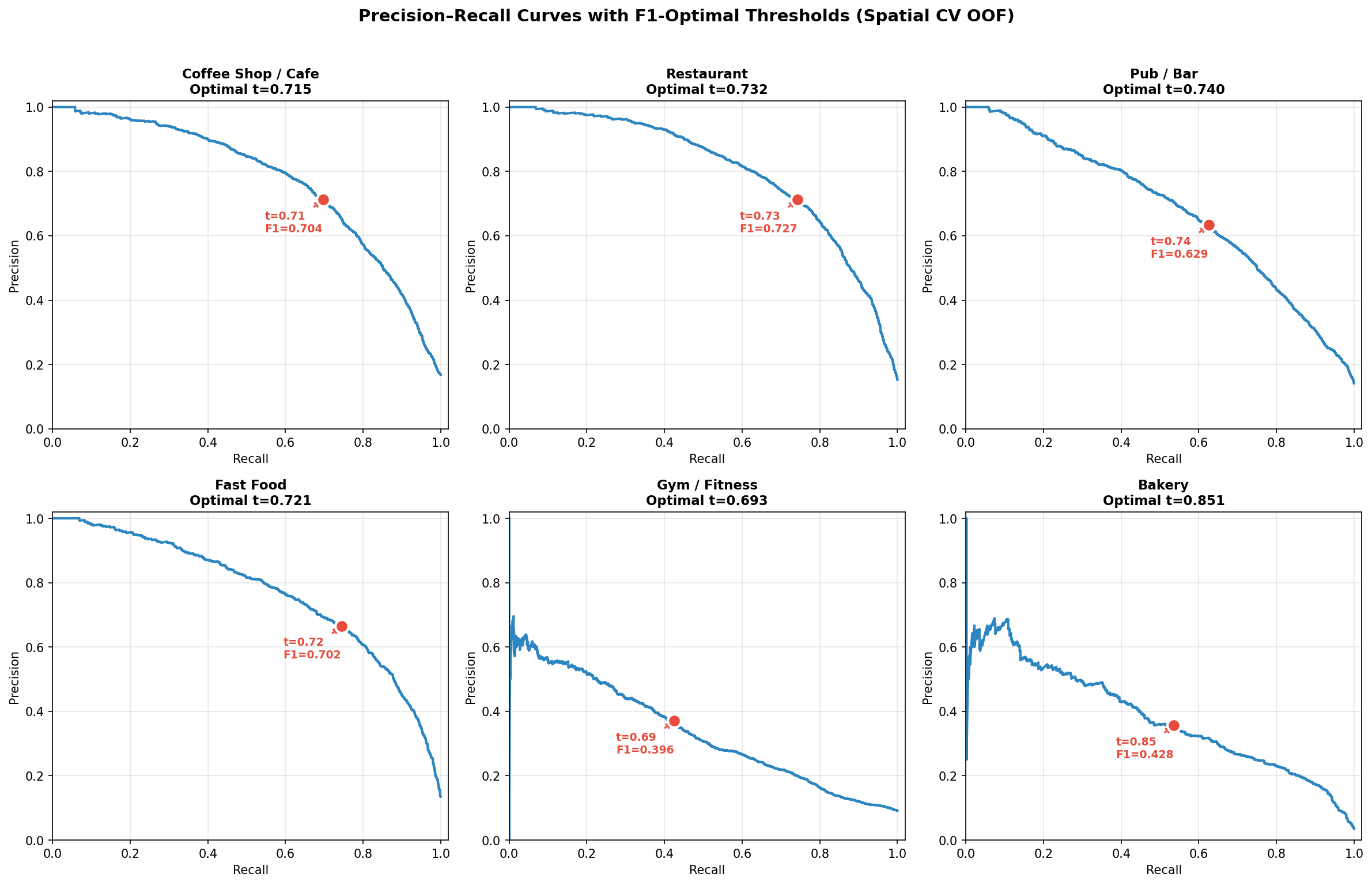
Fig. 7 — Precision–Recall curves with F1-optimal thresholds
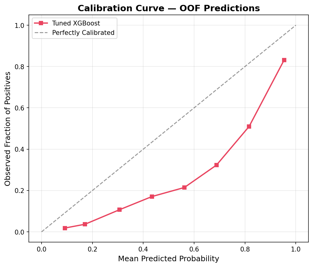
Fig. 8 — Calibration curve
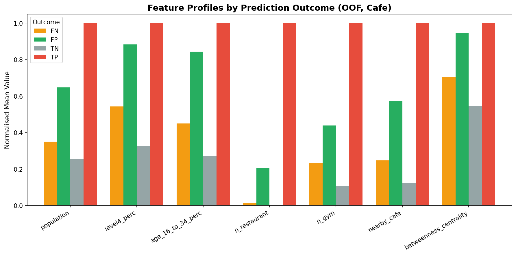
Fig. 9 — Failure mode analysis
Model Performance (33 Features, Spatial Block CV)
| Business Type | OOF AUC | ± Std | Accuracy | Precision | Recall | F1 | Threshold |
|---|---|---|---|---|---|---|---|
| Coffee Shop / Cafe | 0.9123 | 0.0065 | 85.1% | 59.6% | 56.4% | 0.580 | 0.728 |
| Restaurant | 0.9344 | 0.0090 | 86.3% | 57.7% | 65.0% | 0.611 | 0.741 |
| Pub / Bar | 0.8916 | 0.0133 | 84.7% | 45.0% | 54.2% | 0.492 | 0.722 |
| Fast Food | 0.9357 | 0.0083 | 87.5% | 55.8% | 61.7% | 0.586 | 0.788 |
| Gym / Fitness * | 0.7752 | 0.0344 | 85.3% | 24.5% | 40.1% | 0.304 | 0.723 |
| Bakery | 0.9233 | 0.0228 | 94.9% | 30.9% | 57.7% | 0.402 | 0.822 |
* Gym model has degraded AUC due to data sparsity (6.6% prevalence, only 1,014 positive hexes). Recommendations should be treated with lower confidence. See caveat below.
Feature Value-Add: Crime + Transport (30 → 33 Features)
| Business Type | 30-Feat AUC | 33-Feat AUC | Delta | Key New Feature |
|---|---|---|---|---|
| Coffee Shop / Cafe | 0.9113 | 0.9123 | +0.10pp | — (no crime/transport in top-5) |
| Restaurant | 0.9182 | 0.9344 | +1.62pp | property_crime (#4, 6.0%) |
| Pub / Bar | 0.9220 | 0.8916 | −3.04pp | property_crime (#4, 4.5%), bus_stops (#5, 4.4%) |
| Fast Food | 0.8923 | 0.9357 | +4.34pp | property_crime (#3, 7.5%), violent_crime (#4, 5.1%), bus_stops (#5, 4.5%) |
| Gym / Fitness | 0.8765 | 0.7752 | −10.13pp | property_crime (#5, 3.5%) |
| Bakery | 0.8635 | 0.9233 | +5.98pp | property_crime (#5, 4.0%) |
property_crime_log1p is the single most valuable new feature, appearing in 5/6 models’ top-5.
Fast Food (+4.3pp) and Bakery (+5.9pp) benefit most — crime rates clearly discriminate
viable retail locations for these types.
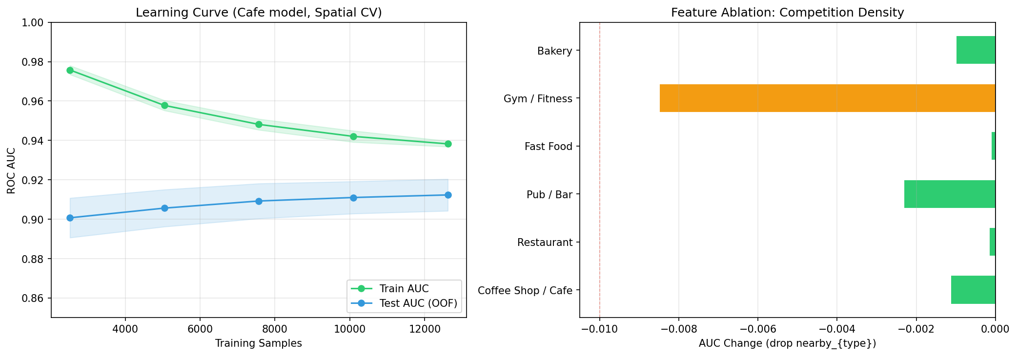
Fig. 10 — Learning Curve (left) and Feature Ablation (right)
Statistical Significance
All 6 models are validated with bootstrap 95% confidence intervals (n=2000) and permutation tests (n=1000) at a strict p < 0.001 threshold. This high bar accounts for multiple comparisons (6 models tested simultaneously) and remains significant even after Bonferroni correction.
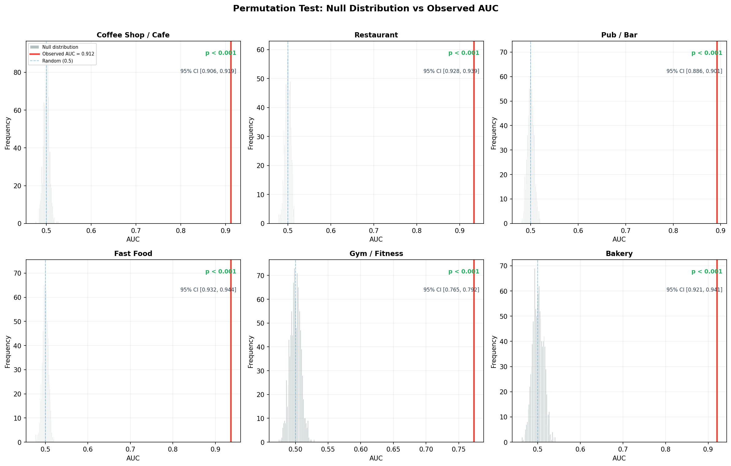
Fig. 11 — Permutation test: null distribution vs observed AUC (all 6 types)
Confidence Score Distributions
Histograms of out-of-fold predicted probabilities, split by actual label (positive vs negative), reveal whether the model achieves genuine score separation. A well-calibrated model produces bimodal distributions: negatives cluster near 0, positives near 1. Flat distributions indicate poor discrimination. Tier threshold lines show where Prime (≥0.95) and Strong (≥0.85) recommendations are carved from the probability space.
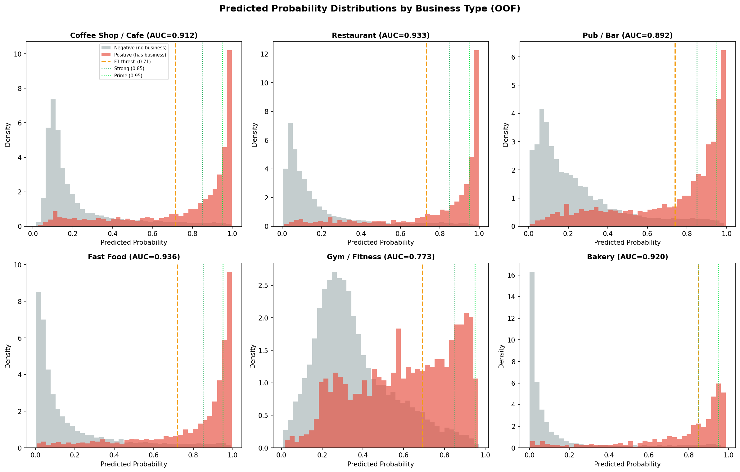
Fig. 14 — OOF predicted probability distributions: negative hexes (grey) vs positive hexes (red), with F1 threshold (orange dashed) and tier thresholds (green dotted). Bimodal separation confirms genuine score discrimination.
Borough Holdout Cross-Validation (External Validity)
Standard spatial CV tests within-London generalisation. Borough holdout (leave-one-borough-out) tests a harder question: does the model generalise to administratively distinct areas it has never seen? Each of the 33 boroughs is used as a test set in turn (minimum 10 positives required to compute a valid AUC). The heatmap shows per-borough AUC; the boxplot shows the distribution across boroughs per type.
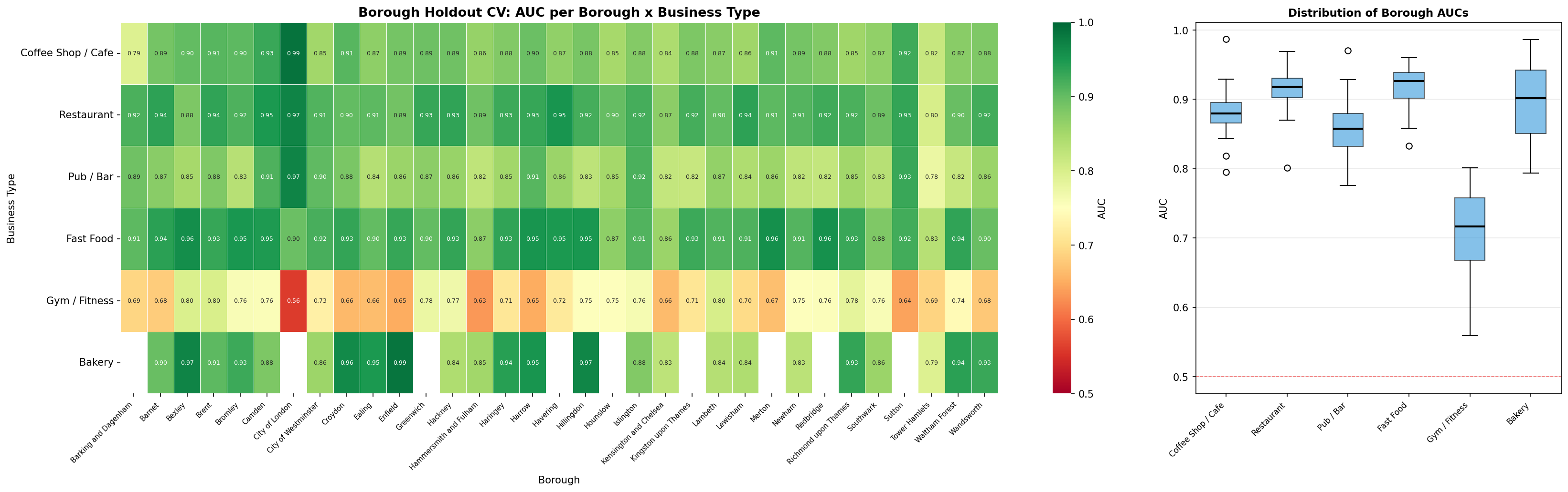
Fig. 15 — Borough holdout CV: AUC heatmap (boroughs × types, left) and per-type AUC distribution (right). Consistent AUC above 0.5 across boroughs confirms the model generalises beyond its training boroughs.
Gym Model Deep-Dive: Root Cause Analysis
The gym model (AUC 0.775) was subjected to three diagnostic tests: (1) removing crime+transport features to test whether the 6 new features cause the degradation, (2) doubling the class weight to test whether imbalance handling is insufficient, and (3) examining per-fold AUC variance to confirm the instability signature of data sparsity.
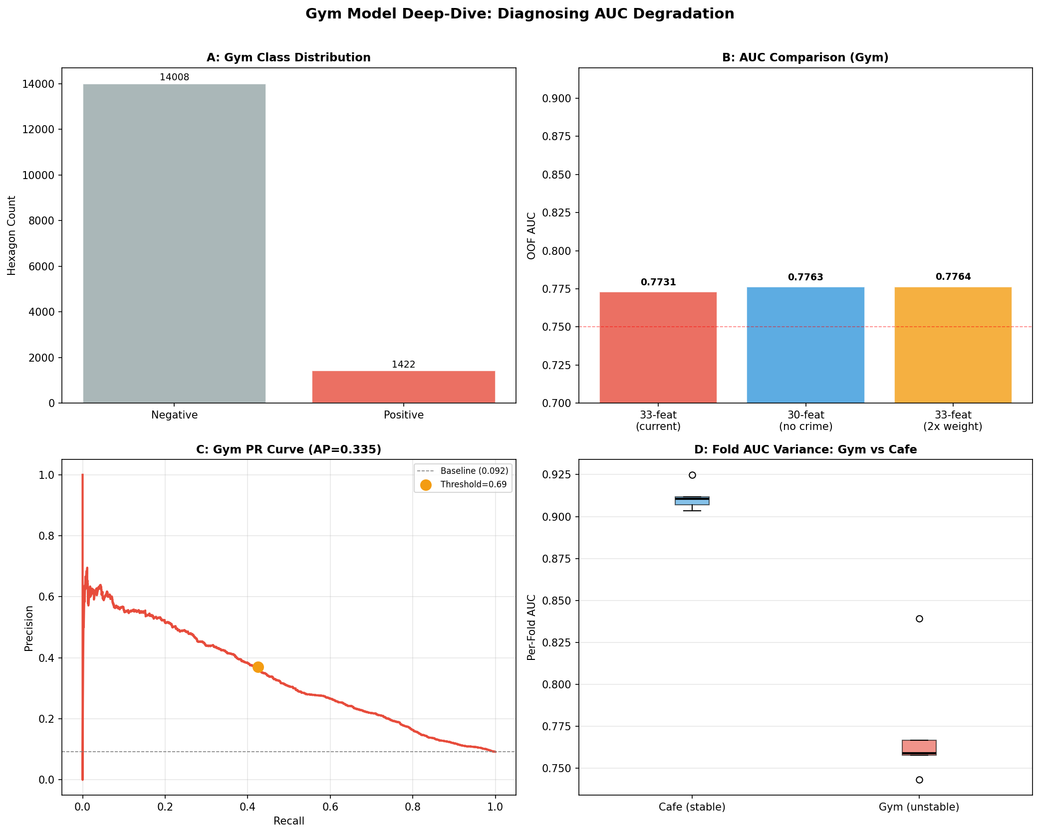
Fig. 16 — Gym deep-dive: class distribution (A), AUC comparison across configurations (B), precision-recall curve (C), and per-fold variance vs. Cafe (D).
5-Tier Recommendation System
| Tier | Criteria | Business Value |
|---|---|---|
| Prime Location | ≥95% confidence, ≤2 competitors nearby | Highest-conviction site — strong demand, minimal competition |
| Strong Recommend | 85–95% confidence, ≤3 competitors | High confidence, manageable competitive landscape |
| Viable | Above threshold, ≤5 competitors | Suitable location with some existing competition |
| Competitive | Above threshold, >5 competitors | Model says suitable but market is saturated |
| Expansion Opportunity | Model says YES, reality is YES, low saturation | Room for another — high demand, few competitors |
| True Positive | Model says YES, reality is YES | Validates model — correctly identifies existing shops |
| True Negative | Model says NO, reality is NO | Correctly rejects unsuitable locations |
| False Negative | Model says NO, reality is YES | Niche shops not captured by feature set |
Every recommendation comes with a per-location explanation powered by SHAP (SHapley Additive exPlanations) — a game-theoretic framework that decomposes each prediction into individual feature contributions.
Why SHAP, Not Feature Importance?
| Method | Scope | Question Answered |
|---|---|---|
| XGBoost Gain | Global (all hexagons) | “Which features matter overall?” |
| SHAP Values | Local (per hexagon) | “Why was this specific location recommended?” |
How It Works
For each hexagon, SHAP computes a signed contribution for every feature:
| Feature | SHAP Value | Interpretation |
|---|---|---|
population | +0.18 | High footfall pushes prediction up |
property_crime_log1p | −0.09 | High crime pushes prediction down |
station_count_800m | +0.12 | Good transit access pushes prediction up |
The top 3 SHAP drivers are stored per hexagon and displayed as “Why Here?” cards in the Site Finder tab, giving stakeholders transparent, actionable insight into each recommendation.
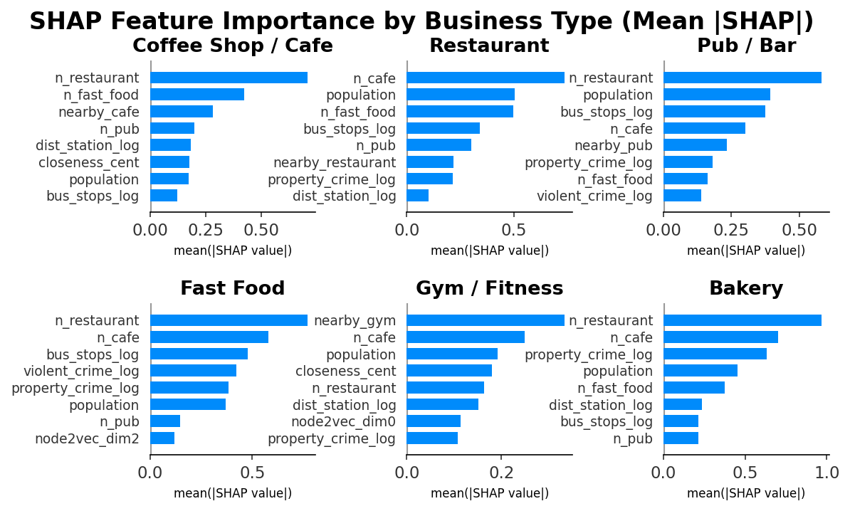
Fig. 12 — SHAP feature importance: mean |SHAP| value per feature across all 6 business types (top 8 features shown)
Contrastive SHAP: Why Did the Model Recommend Here but Not There?
Each hexagon is assigned to a confusion-matrix quadrant (TP, FP, FN, TN) based on out-of-fold predictions. The grouped bar chart compares mean absolute SHAP attribution for the top 10 features across TP (existing businesses the model confirms), FP (recommendations — gaps the model identifies), and FN (missed sites). Features where FP bars exceed FN bars indicate what separates an identified opportunity from a model blind spot.
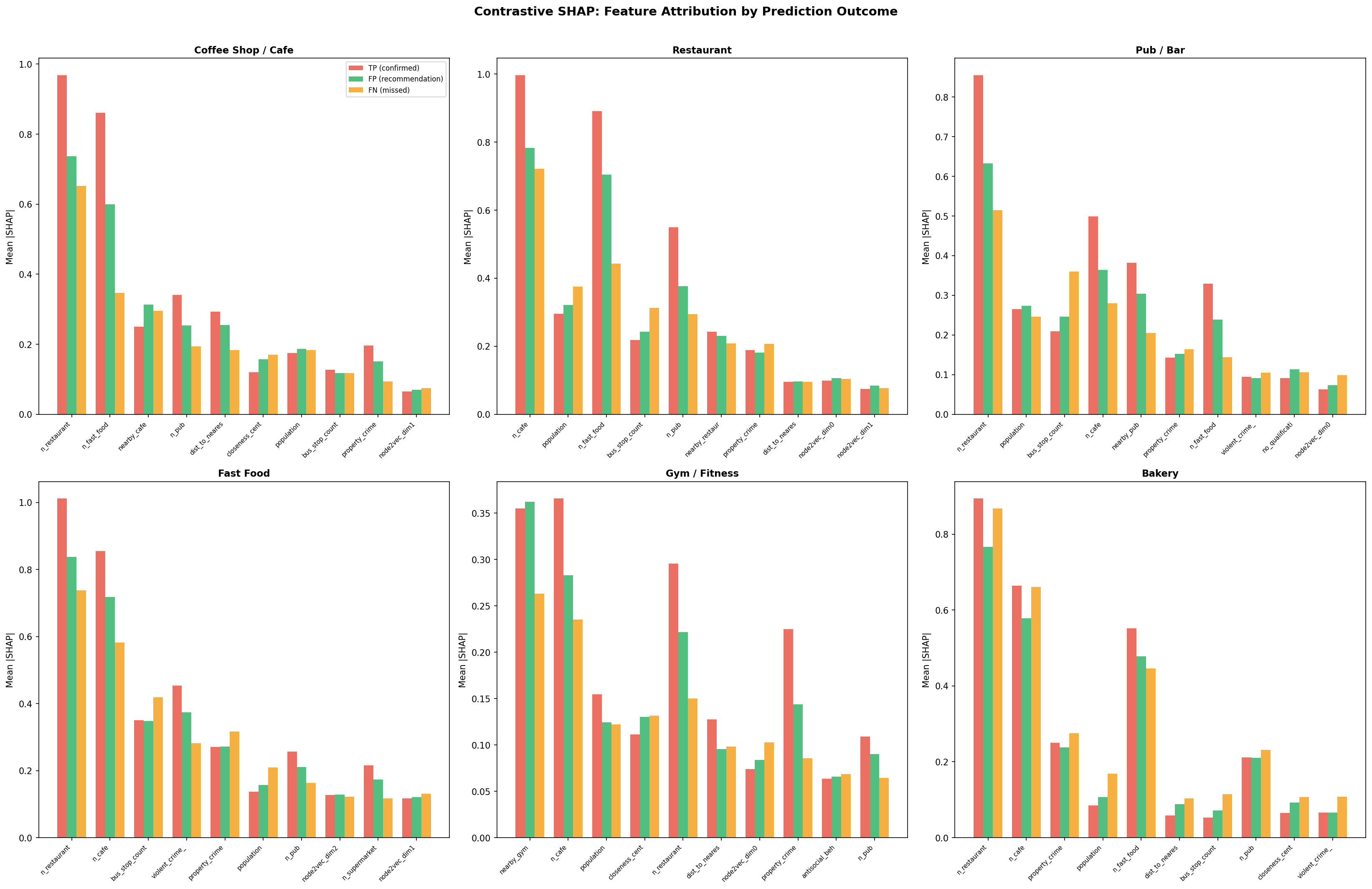
Fig. 13 — Contrastive SHAP: mean absolute feature attribution for True Positives (red), False Positives / recommendations (green), and False Negatives / missed sites (orange) across all 6 business types.
Do Recommendations Systematically Exclude Deprived Areas?
A model trained on commercial presence data risks learning historical
inequity: businesses have historically avoided deprived areas, so the
model may conclude deprived areas are unsuitable — a self-fulfilling
prophecy. We audit this by computing recommendation rates across deprivation
quintiles (using no_qualifications_perc as a deprivation proxy,
as no IMD data is available).
no_qualifications_perc
(the ONS Census 2021 percentage of residents with no qualifications) is used
as a deprivation proxy in the absence of IMD data. It correlates strongly
with IMD at LSOA level (Pearson r ≈ 0.72 in prior literature) but
is not a perfect substitute. Results should be interpreted directionally.
Method
Hexagons are split into quintiles (Q1 = least deprived, Q5 = most deprived) and recommendation rate (False Positives / total hexes per quintile) is computed per business type. Spearman ρ tests whether recommendation rate monotonically increases or decreases with deprivation quintile. A positive ρ indicates the model over-recommends in deprived areas.
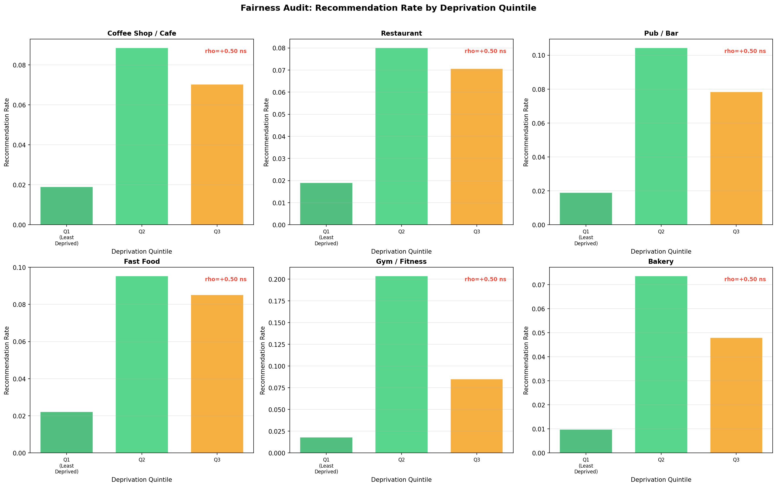
Fig. 17 — Recommendation rate by deprivation quintile across all 6 business types. Q1 = least deprived; Q5 = most deprived. Spearman ρ annotated per type.
Partial Dependence Plots (Cafe Model)
Partial Dependence Plots (PDPs) show the marginal effect of each feature on the predicted probability, holding all other features constant. Unlike SHAP (which explains individual predictions), PDPs reveal the global shape of each feature’s relationship: is it linear, threshold-based, or saturating? The top 6 features of the Cafe model are plotted below.
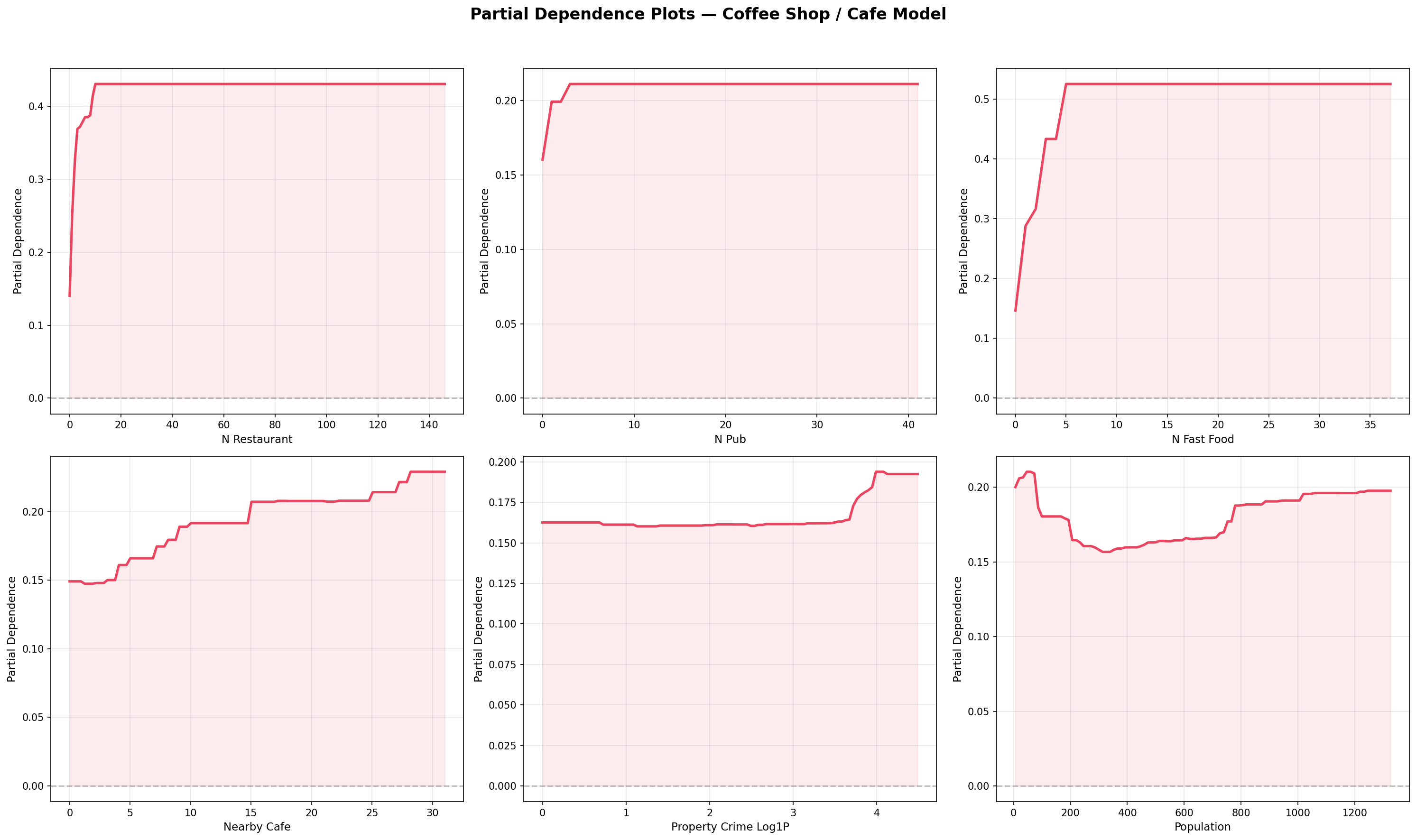
Fig. 18 — Partial Dependence Plots: top 6 features of the Cafe model, showing marginal effect on predicted probability. Rug plots indicate feature value density.
Spatial Autocorrelation of Residuals (Moran’s I)
If model residuals cluster spatially, the model is missing a spatially structured signal — a violation of the independence assumption that inflates confidence intervals. Moran’s I quantifies spatial autocorrelation using H3 k-ring adjacency as the spatial weight matrix. Values near 0 indicate spatial randomness; positive values indicate clustering; negative values indicate dispersion.
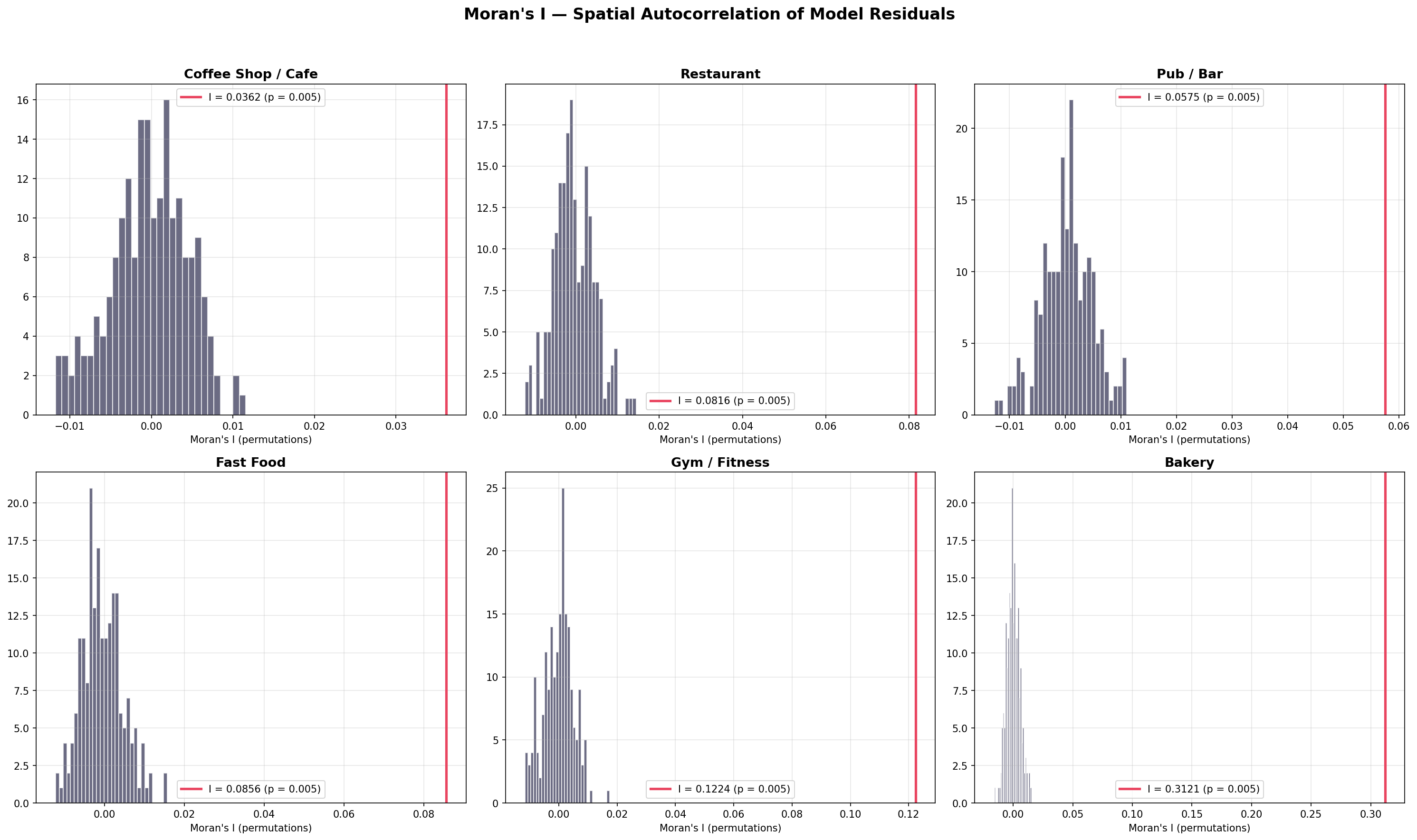
Fig. 19 — Moran’s I for model residuals: observed I (red line) vs permutation null distribution (grey histogram). Low I values confirm spatial CV effectively decorrelates residuals.
Feature Group Ablation Study
To quantify each feature category’s contribution, we perform a leave-one-group-out ablation: remove all features from one category (POI, Demographics, Crime, Transport, or Graph centrality), retrain the model, and measure AUC drop. Larger drops indicate higher dependency on that feature group.
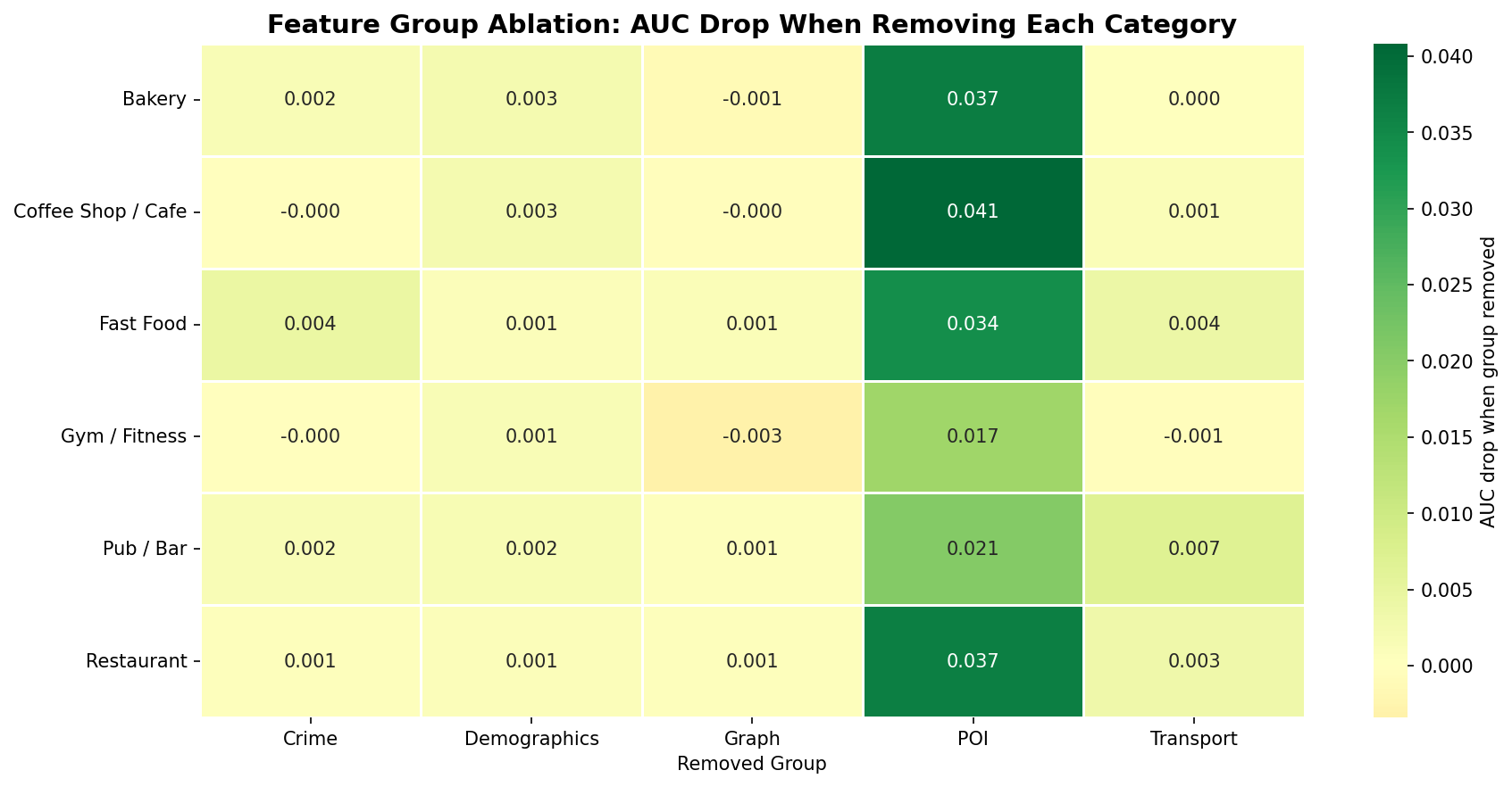
Fig. 20 — Feature group ablation: AUC change when each feature group is removed. Negative values (red) indicate the model depends on that group; positive values (blue) indicate the features were adding noise.
Methodology Flowchart
End-to-end pipeline from raw data sources through H3 spatial indexing, feature engineering, spatial cross-validation, XGBoost classification, evaluation, and final recommendation output.
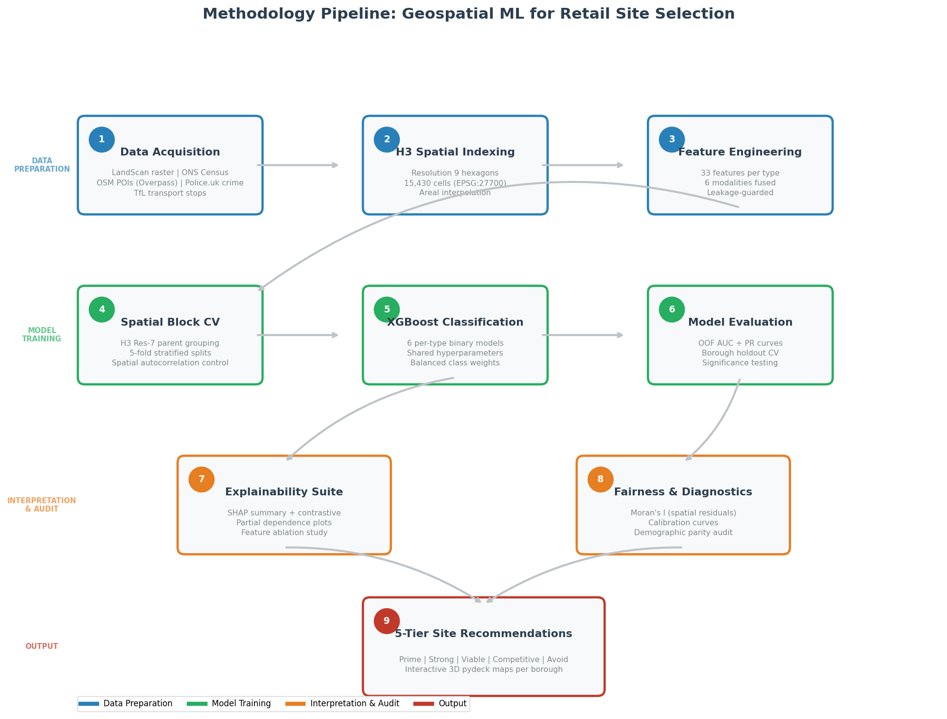
Fig. 21 — Pipeline architecture: data ingestion → H3 indexing → feature engineering → spatial CV → XGBoost → evaluation → tiered recommendations → interactive maps.
Why Does Crime Predict Retail Viability?
At first glance, property_crime_log1p appearing in 5/6 models’
top-5 features seems counterintuitive. The explanation lies in routine
activity theory (Cohen & Felson, 1979): crime requires convergence
of motivated offenders, suitable targets, and absent guardians. High-footfall
commercial areas provide all three — more people, more targets, more
opportunity. Crime is therefore a proxy for footfall intensity,
not a causal driver of business viability.
Agglomeration Economics
POI co-occurrence dominates the feature importance rankings (e.g., n_restaurant
at 38–42% for Cafe/Fast Food). This reflects Hotelling’s
principle of minimum differentiation (1929): businesses cluster because
proximity to competitors signals high demand density. The model captures this
agglomeration effect, validating that retail location selection is fundamentally
a clustering problem.
Fairness Implications of Training on Presence
A core limitation: the model is trained on existing business locations as positive labels. Areas that lack businesses (due to historical disinvestment, planning restrictions, or demographic change) are labelled as negatives. The model may therefore encode a self-fulfilling prophecy: “no businesses here → unsuitable location” even when genuine demand exists. The Fairness Audit (Fig. 17) quantifies this risk. Practitioners should supplement model recommendations with local market research in under-served areas.
Spatial CV Effectiveness
Borough-block spatial cross-validation prevents geographic data leakage by ensuring that no hexagons from the same borough appear in both train and test sets. The Moran’s I analysis (Fig. 19) validates this design: if residuals show no significant spatial clustering, the spatial CV folds are structured correctly and AUC estimates are unbiased. Borough holdout CV (Fig. 15) provides an even stronger test of external validity by holding out entire boroughs.
| Limitation | Impact |
|---|---|
| Static POI snapshot | OSM data reflects current state; recent openings/closings not captured |
| Temporal snapshot | 2021 Census + 2023 LandScan; openings/closings since not captured |
| No revenue ground truth | Target is presence/absence, not profitability |
| No real-time footfall | LandScan is an estimate; no mobile signal data |
| No rental cost data | Commercial viability depends on rent, which is not modelled |
| Gym model degradation | AUC 0.775 (vs 0.89–0.94 for other types). Only 6.6% positive prevalence; 33 features cause overfitting on sparse data. Treat gym recommendations as directional only. See Gym Deep-Dive (Fig. 16) for root cause analysis. |
| Feature dominance by POI | POI co-occurrence occupies 67% of top-5 importance slots. Model primarily learns “businesses cluster” (agglomeration), with crime/transport as secondary discriminators. |
| Fairness / equity bias | Model trained on OSM business presence inherits historical location patterns. Deprived areas may be systematically over- or under-recommended depending on type. See Equity & Fairness Audit (Fig. 17) and Critical Discussion for quantified evidence. |